HealthWorksAI's approach to xAI for Healthcare Payors How does it work?
December 21, 2021 Whitepaper

What's Covered in this Whitepaper
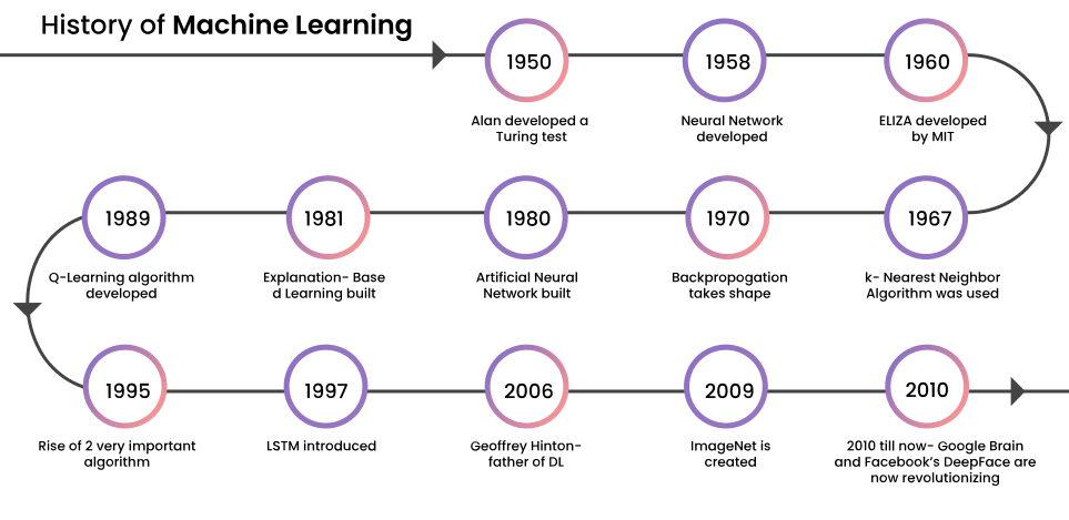
Section 1 – History of AI/ML
Machine Learning (ML) and Artificial Intelligence (AI) have come a long way since the 1950’s when Alan Turing developed the Turing Test, which determined if a computer had human like intelligence, to modern times where computer algorithms can compute complex calculations far beyond human capabilities in an instant.
But while machine learning algorithms have advanced at a rapid rate, so have their complexity. Modern ML algorithms have certainly increased in accuracy, but they also have become harder to explain. While having high accuracy but low explainability can be acceptable for certain requirements like a Netflix recommendation, for highly regulated systems like healthcare, having explainability is crucial. Without explainability we must take the leap to blindly trust the results of complex ML algorithms without knowing the internal decision-making process of the algorithm.
In the context of applied machine learning, the more regulated the vertical, the more challenging it gets to implement advance machine learning. The various techniques, algorithms, and models that are implemented need to be simple and transparent enough to allow for detailed documentation of the internal mechanism. Interpretable, fair, and transparent models are a serious legal mandate in healthcare. Moreover, regulatory regimes are continuously changing, and these regulatory regimes are key drivers of what constitutes interpretability in applied machine learning.
Without interpretability, accountability, and transparency in machine learning decisions, there is no certainty that a machine learning system is not simply relearning and reapplying erroneous human biases. Nor are there any guarantees that we have not designed a machine learning system to make intentionally prejudicial decisions. Hacking and adversarial attacks on machine learning systems are also a serious concern. Without real insight into a complex machine learning system’s operational mechanisms, it can be very difficult to determine whether its outputs have been altered by malicious hacking or whether its inputs can be changed to create unwanted or unpredictable decisions.
With Machine Learning algorithms becoming more complex with time, interpretability is the need of the hour. There is a clear disconnect between how we machines make decisions vs how humans make them, and the fact that machines are making more and more decisions for us, has birthed a new push for transparency and a field of research called Explainable AI, or xAI whose goal is to make machines able to account for the things they learn, in ways that we can understand.
Section 2 – What is xAI?
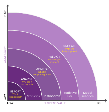
Many machine learning algorithms have been labeled “black box” models because of their inscrutable inner workings. What makes these models accurate is what makes their predictions difficult to understand: they are very complex. This is a fundamental trade-off. These algorithms are typically more accurate for predicting non-linear, faint, or rare phenomena. Unfortunately, more accuracy almost always comes at the expense of interpretability, and interpretability is crucial for business adoption, model documentation, regulatory oversight, and human acceptance and trust.

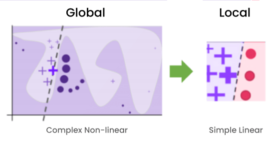
In the graph above we can see this trade off. Simple linear models that can be easily interpreted by humans but might not have very accurate predictions for complex problems. On the other hand, highly non-linear models provide very high accuracy but are too complex for humans to understand.
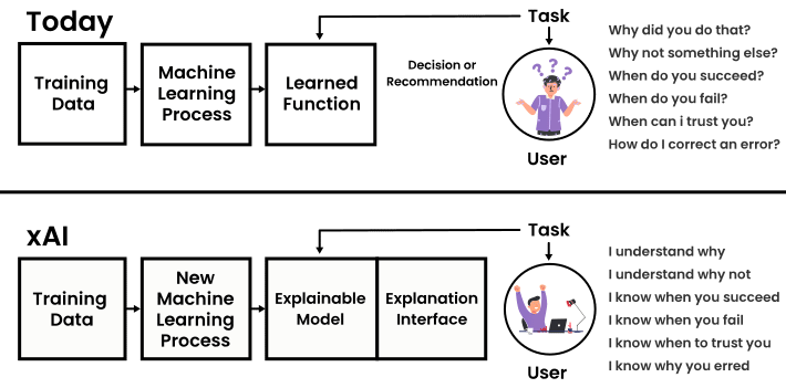
The xAI concept can be best explained using the below image. While advanced machine learning algorithms certainly provide results, knowing how we got these results or how can we tweak these results is nearly impossible because of the black box conundrum. On the other hand, by introducing xAI as an explainable model we can not only understand how we got these results but are now in a position to tweak the model.
Section 3 – How do we go about an xAI exercise?
- Either the model can be easily interpreted (model based)
- Or derive human understandable explanations (post-hoc)
- Black box approach – we do not know anything about the inside working of the model.
- Whitebox approach – we have access to model’s internal workings.
- Model agnostic interpretable methods – applicable to all model types.
- Model specific interpretable methods – applicable only to specific model types.
- Global Explanation – interpretable methods that try to explain the whole model.
- Local Explanation – interpretable methods that explain parts of the model like individual predictions.
- Graph
- Image
- Text/speech
- Tabular
- Visual
- Feature importance
- Data points
- Surrogate models
Section 4 – Importance of interpretable ML in healthcare and the HealthWorksAI approach to Product Lifecycle Management
Product Lifecycle Management (PLM) is a long-term game. There is no secret solution to package the best benefit structure while doubling one’s market share simultaneously. It’s a long-term iterative process and each market is unique and evolves at a different rate.
Data is a byproduct of operations. Organizations are starving for insights while drowning in data. While everyone agrees that it vital to convert raw data to actionable insights, to blindly trust the results of advanced modeling techniques can be detrimental in the Product Lifecycle Management.
The design of any plan requires multiple iterations between the product team and the actuary team, with each having their own list of qualifications that defines a successful plan design. Product teams will always wish to add as many benefits as they can to maximize enrollments while the actuary team will always focus on viability and profitability.
- Product design
- Marketing
- Provider Network
Level 1 – assign each plan a TPV (True Plan Value) and a product score. This way we can see how valuable each plan is to the eyes of the beneficiary when compared to Original Medicare.
What is TPV?
The HealthWorksAI True Plan Value (TPV), the value realized by the member, includes the cost of offering non-Medicare covered benefits, such as vision, dental, fitness, OTC. It also covers the cost of the buy down of member cost sharing that would have accrued to member under Original Medicare.
Level 2 – using advanced analytics segment factors/benefits as significant and insignificant in their markets. Also, identity the benefits that are “Table Stakes” which are defined as the benefits that are provided by nearly every plan and are considered the bare minimum a plan must offer to be considered as a competitive plan.
Level 3 – using advanced analytics, we can start to go a level deeper and begin to simulate benefit design and see how the various changes in the plan structure will affect enrollment gains.
Having a robust provider network is key to keeping beneficiaries happy. With a healthy number of PCPs and specialists, beneficiaries need not worry about having to consult a physician or specialist outside of their network. However, while having a higher number of PCPs or specialist in a network may translate to a strong network, having a smaller network with higher quality NPIs is an equally good option. Healthworks breaks the Provider Network analysis into the following levels.
Level 1 – Assign a provider network score, to each network. This score allows a comparison of payer-provider networks in a region.
What is the provider score?
The provider score is a proprietary HWAI single metric that allows comparison of payer provider networks.
How is it created?
Using rule-based modeling techniques, appropriated weightages are applied to the composition, strength, and the quality of network by looking at hospitals, PCPs and specialists in the network. We also apply a proprietary indexing to the providers that calibrates the influence of the NPI in the market – this index also feeds into the provider network score.
Level 2 – Allow payers to compare the PCP, hospital & specialist counts of their networks with their competitor networks.
Level 3 – Apply proprietary indexing to providers that calibrate the influence of the NPI in the market. This provider index helps payers develop smaller competitive networks which perform better than competitor networks.
Marketing is very crucial for Medicare Advantage marketing teams because it is the last step before plans go live during AEP. For marketing teams to continue to perform with the same capacity coupled with replicating YoY enrollment gains they need to ensure that they spend the right amount in the right channels. But determining the right amounts for each channel can get tricky and with every dollar being spent coming under such high scrutiny, finding ways to optimize spends is the need of the hour.
Level 1 – Provide a marketing score to each organization by computing all their spends across multiple channels into a single integrated platform.
What is the marketing score?
The marketing score is a proprietary HWAI single metric that allows comparison of payer marketing efforts that resonates with the beneficiaries.
How is it created?
Using NN-based modeling techniques, the relative importance/impact of the various channel spends, messaging, target market and the timing are analyzed for the different plan types. We also apply a proprietary indexing to the marketing that calibrates the influence of the brand in the market – this index also feeds into the marketing score.
Level 2 – using advanced analytics segment the marketing channels as significant and insignificant and provide the weightage of each channel on enrollment gains.
Level 3 – once we know which channels are the most important, we can use advanced analytics to optimize spends and increase ROIs using simulators.
Each level for all the three categories involves advanced data analytic techniques with xAI methodologies coupled with a sound business knowledge foundation. But the use of xAI is most important during the segmentation of factors. Through xAI we can better understand what features are the most important during segmentation which can be verified by extensive EDA and business knowledge.
Section 5 – The HealthWorksAI approach to xAI
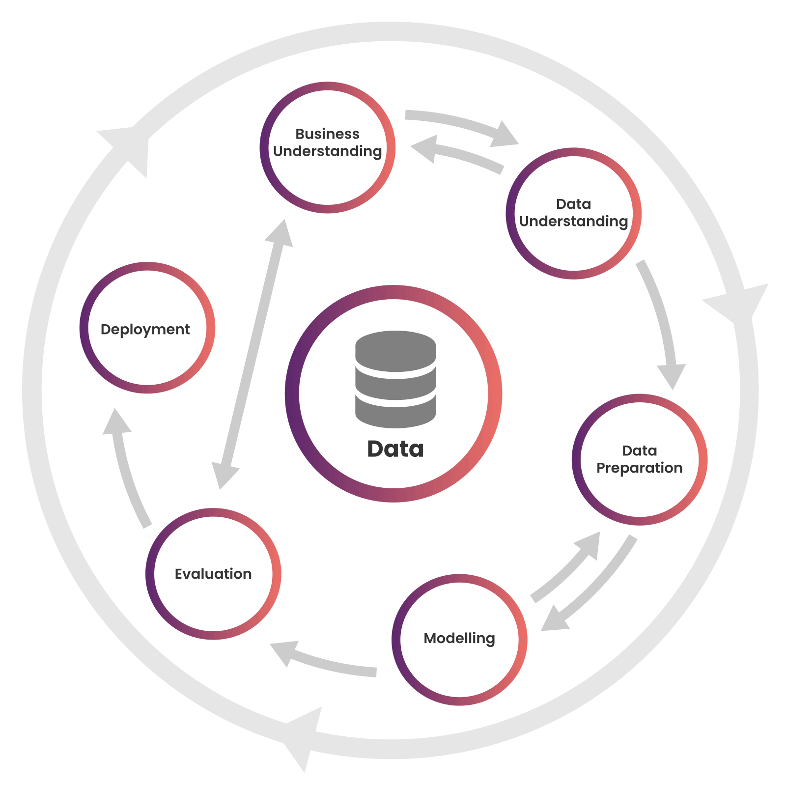
At HealthWorks we use the Cross-industry standard process for data mining, known as CRISP-DM for data mining, a process model with six phases that naturally describes the data science life cycle. It’s like a set of guardrails to help you plan, organize, and implement your data science (or machine learning) project. CRISP-DM breaks the process of data mining into six major phases –
- What does the client need & what are they trying to accomplish?
- Define what a successful plan is to the client.
- Produce project planner. This involves a detailed plan for each phase of the project.
- What does the client need & what are they trying to accomplish?
- Define what a successful plan is to the client.
- Produce project planner. This involves a detailed plan for each phase of the project.
- How do we organize the data for modeling?
- Which rows/columns do we exclude?
- Do we have multiple data sources? How do we correctly integrate all data sets?
- Data formatting. Are all the columns in the right format before we start the modelling exercise?
- Modeling techniques selection. Which methodology best suits our needs?
- Divide the data into a training a test data sets.
- Build and assess model results.
- Which model best meets the business objectives?
- Do we need to repeat any of the previous steps?
- Summarize findings.
- Finetune and document the entire process so it can be easily replicated.
- Provide the results to the stakeholders.
- Project review. See what could have been improved to ensure a more streamlined process in the future.
In the CRISP-DM cycle, advanced analytics & xAI comes to play in the modeling and evaluation phases. Using only one set of ML algorithms to get the required results is perfectly acceptable, however, using multiple algorithms and models coupled with advanced model ensembling techniques allows us to achieve far superior results. At HealthWorks we use a combination of Rule based modeling, Random Forest, and Artificial Neural Networks to develop our proprietary prediction, classification, and performance metrics. And while these modeling techniques yield results with high accuracy, they are in essence black box models.
To better understand these models, we need to be able to look inside the black box and decode the results using xAI methodologies. To achieve this, we use LIME and DeepLIFT.
LIME stands for Local Interpretable Model Agnostic Explanation and is one of the most popular xAI methodologies for black box models. LIME gives explanations that are locally faithful within the boundries of the observation/sample being explained.
the three basic ideas behind this explanation method:
- Model-agnosticism. In other words, model-independent, which means that LIME doesn’t make any assumptions about the model whose prediction is explained. It treats the model as a black-box, so the only way that it has to understand its behavior is perturbing the input and see how the predictions change.
- Interpretability. Explanations need to be easy to understand by users above all, which is not necessarily true for the feature space used by the model because it may use too many input variables (even a linear model can be difficult to interpret if it has hundreds or thousands of coefficients) or it simply uses too complex/artificial variables (and explanations in terms of these variables will not be interpretable by a human). For this reason, LIME’s explanations use a data representation (called interpretable representation) that is different from the original feature space.
- Locality. LIME produces an explanation by approximating the black-box model by an interpretable model (for example, a linear model with a few non-zero coefficients) in the neighborhood of the instance we want to explain.
To ensure that the explanation is interpretable, LIME distinguishes an interpretable representation from the original feature space that the model uses. The interpretable representation must be understandable to humans, so its dimension is not necessarily the same as the dimension of the original feature space.
Let p be the dimension of the original feature space X and let p’ be the dimension of the interpretable space X’. The interpretable inputs map to the original inputs through a mapping function hʸ: X’→X, specific to the instance we want to explain y∈ X.
For tabular data (i.e., matrices), the interpretable representation depends on the type of features: categorical, numerical or mixed data. For categorical data, X’={0,1}ᵖ where p is the actual number of features used by the model (i.e., p’=p) and the mapping function maps 1 to the original class of the instance and 0 to a different one sampled according to the distribution of training data. For numerical data, X’=X and the mapping function is the identity. However, we can discretize numerical features so that they can be considered categorical features. For mixed data, the interpretable representation will be a p-dimensional space composed of both binary features corresponding to categorical features and numerical features corresponding to numerical features (if they are not discretized). Each component of the mapping function is also defined according to the previous definitions depending on the type of the explanatory variable.
Let 𝔏(f,g,wʸ) be a loss function that measures how unfaithful g is in approximating f in the locality defined by wʸ, and let Ω(g) be a measure of complexity of the explanation g∈ G.
In order to ensure both interpretability and local fidelity, we must minimize 𝔏(f,g,wʸ) while having Ω(g) be low enough to be interpretable by humans. Thus, the explanation ξ(y) produced by LIME is obtained by the following:
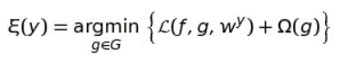
Note that this formulation can be used with different explanation families G, loss functions 𝔏 and regularization terms Ω.
In practice, the general approach LIME uses to produce an explanation is the following:
- Generate N “perturbed” samples of the interpretable version of the instance to explain y’. Let {zᵢ’∈X’ | i=1,…,N} be the set of these observations.
- Recover the “perturbed” observations in the original feature space by means of the mapping function. Let {zᵢ ≡ hʸ(zᵢ’)∈X | i=1,…,N} be the set in the original representation.
- Let the black box model predict the outcome of every “perturbed” observation. Let {f(zᵢ)∈ℝ | i=1,…,N} be the set of responses.
- Compute the weight of every “perturbed” observation. Let {wʸ(zᵢ)∈ℝ⁺ | i=1,…,N} be the set of weights.
- Select K features best describing the black box model outcome from the perturbed dataset ℨ.
- Fit a weighted linear regression model (actually, current implementations of LIME fit a weighted ridge regression with the regularization parameter set to 1) to a feature-reduced dataset composed of the K selected features in step 5. If the black box model is a regressor, the linear model will predict the output of the black box model directly. If the black box model is a classifier, the linear model will predict the probability of the chosen class.
- Extract the coefficients from the linear model and use them as explanations for the black box model’s local behavior.
Note that the complexity does not depend on the size of the training set (because it produces the explanation for an individual prediction), but instead on time to compute predictions f(z) and on the number of samples N.
For tabular data (i.e., matrices), there are differences between categorical and numerical features, but both types are dependent on the training set. For categorical features (whose interpretable representation is binary) perturbed samples are obtained by sampling according to the training distribution and making a binary feature that is 1 when the value is the same as the instance being explained. For numerical features, the instance being explained is perturbed by sampling from a Normal(0,1) distribution and doing the inverse operation of mean-centering and scaling (using the means and standard deviations of the training data).
DeepLIFT is a relatively new methodology and is primarily used for neural networks for audio and visual inputs.
Compositional models such as deep neural networks are comprised of many simple components. Given analytic solutions for the Shapley values of the components, fast approximations for the full model can be made using DeepLIFT’s style of back-propagation.
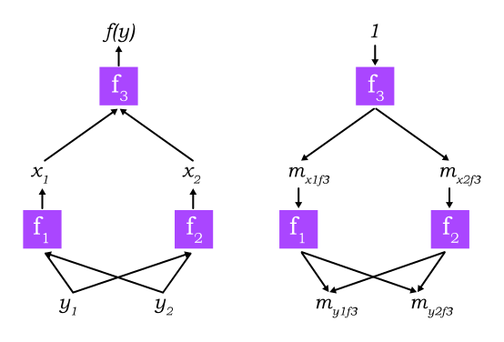
Since DeepLIFT is an additive feature attribution method that satisfies local accuracy and missingness, we know that Shapley values represent the only attribution values that satisfy consistency. This motivates our adapting DeepLIFT to become a compositional approximation of SHAP values, leading to Deep SHAP. Deep SHAP combines SHAP values computed for smaller components of the network into SHAP values for the whole network. It does so by recursively passing DeepLIFT’s multipliers, now defined in terms of SHAP values, backwards through the network as shown in the above image.
Since the SHAP values for the simple network components can be efficiently solved analytically if they are linear, max pooling, or an activation function with just one input, this composition rule enables a fast approximation of values for the whole model. Deep SHAP avoids the need to heuristically choose ways to linearize components. Instead, it derives an effective linearization from the SHAP values computed for each component.
Section 6 – Conclusion
With rapid advancements in AI/ML algorithms we certainly are heading towards an analytical based future. But the more we advance the further we step into a black box future. While xAI might not be the need of the hour, we are consistently getting more dependent on complex AI/ML algorithms, and by investing time into xAI solutions today we can ensure we are ahead of our competition in the future.
References
- https://research.aimultiple.com/xai/
- https://www.sciencedirect.com/science/article/pii/S1566253519308103
- https://www.geeksforgeeks.org/introduction-to-explainable-aixai-using-lime/
- https://www.analyttica.com/demystifying-lime-xai-through-leaps/
- https://pythondata.com/local-interpretable-model-agnostic-explanations-lime-python/
- https://towardsdatascience.com/lime-how-to-interpret-machine-learning-models-with-python-94b0e7e4432e
- https://coderzcolumn.com/tutorials/machine-learning/how-to-use-lime-to-understand-sklearn-models-predictions#LIME—Local-Interpretable-Model-Agnostic-Explanations-
- https://arxiv.org/pdf/1704.02685.pdf
- https://mrsalehi.medium.com/a-review-of-different-interpretation-methods-in-deep-learning-part-2-input-gradient-layerwise-e077609b6377
- https://towardsdatascience.com/explainable-neural-networks-recent-advancements-part-3-6a838d15f2fb
- https://towardsdatascience.com/understanding-how-lime-explains-predictions-d404e5d1829c
- http://www.columbia.edu/~jwp2128/Papers/IbrahimLouieetal2019.pdf
- https://christophm.github.io/interpretable-ml-book/shap.html
- https://proceedings.neurips.cc/paper/2017/file/8a20a8621978632d76c43dfd28b67767-Paper.pdf
- https://blog.fiddler.ai/2021/02/the-past-present-and-future-states-of-explainable-ai/